Time series forecasting with ARMA and InfluxDB

An ARMA or autoregressive moving average model is a forecasting model that predicts future values based on past values. Forecasting is a critical task for several business objectives, such as predictive analytics, predictive maintenance, product planning, budgeting, etc. A big advantage of ARMA models is that they are relatively simple. They only require a small dataset to make a prediction, they are highly accurate for short forecasts, and they work on data without a trend.

In this tutorial, we’ll learn how to use the Python statsmodels package to forecast data using an ARMA model and InfluxDB, the open source time series database. The tutorial will outline how to use the InfluxDB Python client library to query data from InfluxDB and convert the data to a Pandas DataFrame to make working with the time series data easier. Then we’ll make our forecast.

I’ll also dive into the advantages of ARMA in more detail.

Requirements

This tutorial was executed on a macOS system with Python 3 installed via Homebrew. I recommend setting up additional tooling like virtualenv, pyenv, or conda-env to simplify Python and client installations. Otherwise, the full requirements are here:

• influxdb-client = 1.30.0
• pandas = 1.4.3
• influxdb-client >= 1.30.0
• pandas >= 1.4.3
• matplotlib >= 3.5.2
• sklearn >= 1.1.1

This tutorial also assumes that you have a free tier InfluxDB cloud account and that you have created a bucket and created a token. You can think of a bucket as a database or the highest hierarchical level of data organization within InfluxDB. For this tutorial we’ll create a bucket called NOAA.

What is ARMA?

ARMA stands for auto-regressive moving average. It’s a forecasting technique that is a combination of AR (auto-regressive) models and MA (moving average) models. An AR forecast is a linear additive model. The forecasts are the sum of past values times a scaling factor plus the residuals. To learn more about the math behind AR models, I suggest reading this article.

A moving average model is a series of averages. There are different types of moving averages including simple, cumulative, and weighted forms. ARMA models combine the AR and MA techniques to generate a forecast. I recommend reading this post to learn more about AR, MA, and ARMA models. Today we’ll be using the statsmodels ARMA function to make forecasts.

Assumptions of AR, MA, and ARMA models

If you’re looking to use AR, MA, and ARMA models then you must first make sure that your data meets the requirements of the models: stationarity. To evaluate whether or not your time series data is stationary, you must check that the mean and covariance remain constant. Luckily we can use InfluxDB and the Flux language to obtain a dataset and make our data stationary.

We’ll do this data preparation in the next section.

Flux for time series differencing and data preparation

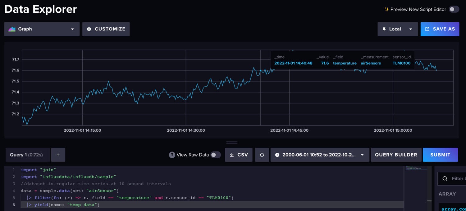
Flux is the data scripting language for InfluxDB. For our forecast, we’re using the Air Sensor sample dataset that comes out of the box with InfluxDB. This dataset contains temperature data from multiple sensors. We’re creating a temperature forecast for a single sensor. The data looks like this:

InfluxData

Use the following Flux code to import the dataset and filter for the single time series.

 
import "join"
import "influxdata/influxdb/sample"
//dataset is regular time series at 10 second intervals
data = sample.data(set: "airSensor")
  |> filter(fn: (r) => r._field == "temperature" and r.sensor_id == "TLM0100")

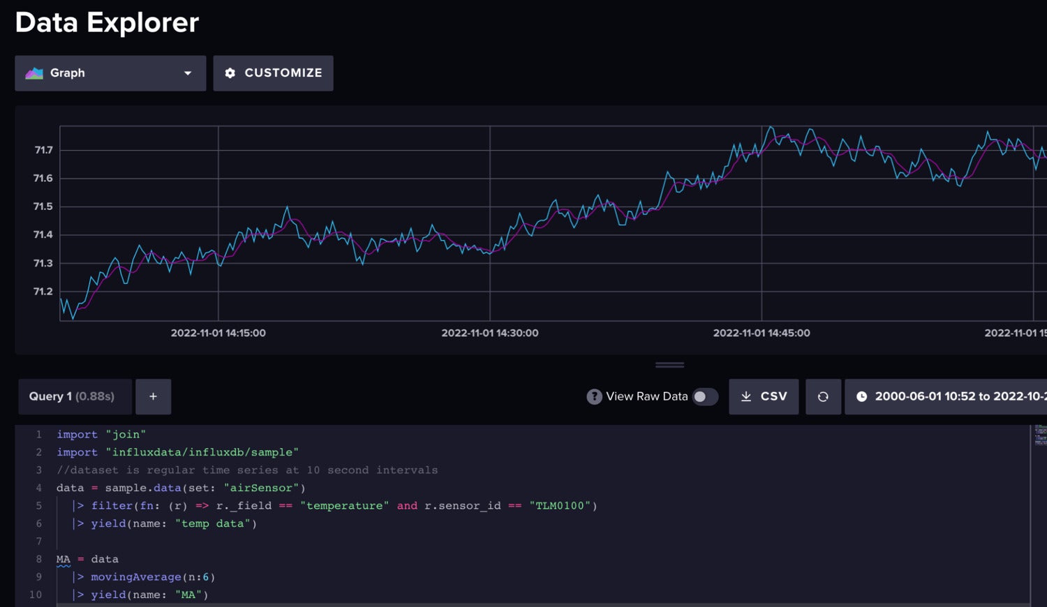
Next we can make our time series weakly stationary by differencing the moving average. Differencing is a technique to remove any trend or slope from our data. We will use moving average differencing for this data preparation step. First we find the moving average of our data.

InfluxData

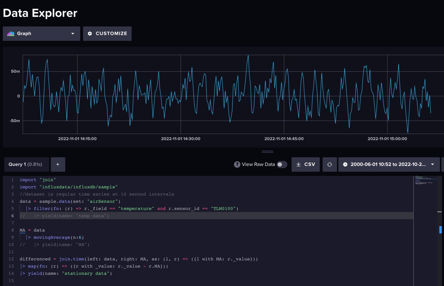
Next we subtract the moving average from our actual time series after joining the raw data and MA data together.

InfluxData

Here is the entire Flux script used to perform this differencing:

 
import "join"
import "influxdata/influxdb/sample"
//dataset is regular time series at 10 second intervals
data = sample.data(set: "airSensor")
  |> filter(fn: (r) => r._field == "temperature" and r.sensor_id == "TLM0100")
//   |> yield(name: "temp data")

MA = data
  |> movingAverage(n:6)
//   |> yield(name: "MA")

differenced = join.time(left: data, right: MA, as: (l, r) => (l with MA: r._value))
|> map(fn: (r) => (r with _value: r._value - r.MA))
|> yield(name: "stationary data")

Please note that this approach estimates the trend cycle. Series decomposition is often performed with linear regression as well.

ARMA and time series forecasts with Python

Now that we’ve prepared our data, we can create a forecast. We must identify the p value and q value of our data in order to use the ARMA method. The p value defines the order of our AR model. The q value defines the order of the MA model. To convert the statsmodels ARIMA function to an ARMA function we provide a d value of 0. The d value is the number of nonseasonal differences needed for stationarity. Since we don’t have seasonality we don’t need any differencing.

First we query our data with the Python InfluxDB client library. Next we convert the DataFrame to an array. Then we fit our model, and finally we make a prediction.

 
# query data with the Python InfluxDB Client Library and remove the trend through differencing
client = InfluxDBClient(url="https://us-west-2-1.aws.cloud2.influxdata.com", token="NyP-HzFGkObUBI4Wwg6Rbd-_SdrTMtZzbFK921VkMQWp3bv_e9BhpBi6fCBr_0-6i0ev32_XWZcmkDPsearTWA==", org="0437f6d51b579000")
# write_api = client.write_api(write_options=SYNCHRONOUS)
query_api = client.query_api()
df = query_api.query_data_frame('import "join"'
'import "influxdata/influxdb/sample"'
'data = sample.data(set: "airSensor")'
  '|> filter(fn: (r) => r._field == "temperature" and r.sensor_id == "TLM0100")'
'MA = data'
  '|> movingAverage(n:6)'
'join.time(left: data, right: MA, as: (l, r) => (l with MA: r._value))'
'|> map(fn: (r) => (r with _value: r._value - r.MA))'
'|> keep(columns:["_value", "_time"])'
'|> yield(name:"differenced")'
)
df = df.drop(columns=['table', 'result'])
y = df["_value"].to_numpy()
date = df["_time"].dt.tz_localize(None).to_numpy()
y = pd.Series(y, index=date)
model = sm.tsa.arima.ARIMA(y, order=(1,0,2))
result = model.fit()

Ljung-Box test and Durbin-Watson test

The Ljung-Box test can be used to verify that the values you used for p,q for fitting an ARMA model are good. The test examines autocorrelations of the residuals. Essentially it tests the null hypothesis that the residuals are independently distributed. When using this test, your goal is to confirm the null hypothesis or show that the residuals are in fact independently distributed. First you must fit your model with chosen p and q values, like we did above. Then use the Ljung-Box test to determine if those chosen values are acceptable. The test returns a Ljung-Box p-value. If this p-value is greater than 0.05, then you have successfully confirmed the null hypothesis and your chosen values are good.

After fitting the model and running the test with Python…

print(sm.stats.acorr_ljungbox(res.resid, lags=[5], return_df=True))

we get a p-value for the test of 0.589648.

lb_stat	lb_pvalue
5  3.725002	0.589648

This confirms that our p,q values are acceptable during model fitting.

You can also use the Durbin-Watson test to test for autocorrelation. Whereas the Ljung-Box tests for autocorrelation with any lag, the Durbin-Watson test uses only a lag equal to 1. The result of your Durbin-Watson test can vary from 0 to 4 where a value close to 2 indicates no autocorrelation. Aim for a value close to 2.

print(sm.stats.durbin_watson(result.resid.values))

Here we get the following value, which agrees with the previous test and confirms that our model is good.

2.0011309357716414

Complete ARMA forecasting script with Python and Flux

Now that we understand the components of the script, let’s look at the script in its entirety and create a plot of our forecast.

 
import pandas as pd
import numpy as np
import matplotlib.pyplot as plt
from influxdb_client import InfluxDBClient
from datetime import datetime as dt
import statsmodels.api as sm
from statsmodels.tsa.arima.model import ARIMA
# query data with the Python InfluxDB Client Library and remove the trend through differencing
client = InfluxDBClient(url="https://us-west-2-1.aws.cloud2.influxdata.com", token="NyP-HzFGkObUBI4Wwg6Rbd-_SdrTMtZzbFK921VkMQWp3bv_e9BhpBi6fCBr_0-6i0ev32_XWZcmkDPsearTWA==", org="0437f6d51b579000")
# write_api = client.write_api(write_options=SYNCHRONOUS)
query_api = client.query_api()
df = query_api.query_data_frame('import "join"'
'import "influxdata/influxdb/sample"'
'data = sample.data(set: "airSensor")'
  '|> filter(fn: (r) => r._field == "temperature" and r.sensor_id == "TLM0100")'
'MA = data'
  '|> movingAverage(n:6)'
'join.time(left: data, right: MA, as: (l, r) => (l with MA: r._value))'
'|> map(fn: (r) => (r with _value: r._value - r.MA))'
'|> keep(columns:["_value", "_time"])'
'|> yield(name:"differenced")'
)
df = df.drop(columns=['table', 'result'])
y = df["_value"].to_numpy()
date = df["_time"].dt.tz_localize(None).to_numpy()
y = pd.Series(y, index=date)
model = sm.tsa.arima.ARIMA(y, order=(1,0,2))
result = model.fit()
fig, ax = plt.subplots(figsize=(10, 8))
fig = plot_predict(result, ax=ax)
legend = ax.legend(loc="upper left")
print(sm.stats.durbin_watson(result.resid.values))
print(sm.stats.acorr_ljungbox(result.resid, lags=[5], return_df=True))
plt.show()

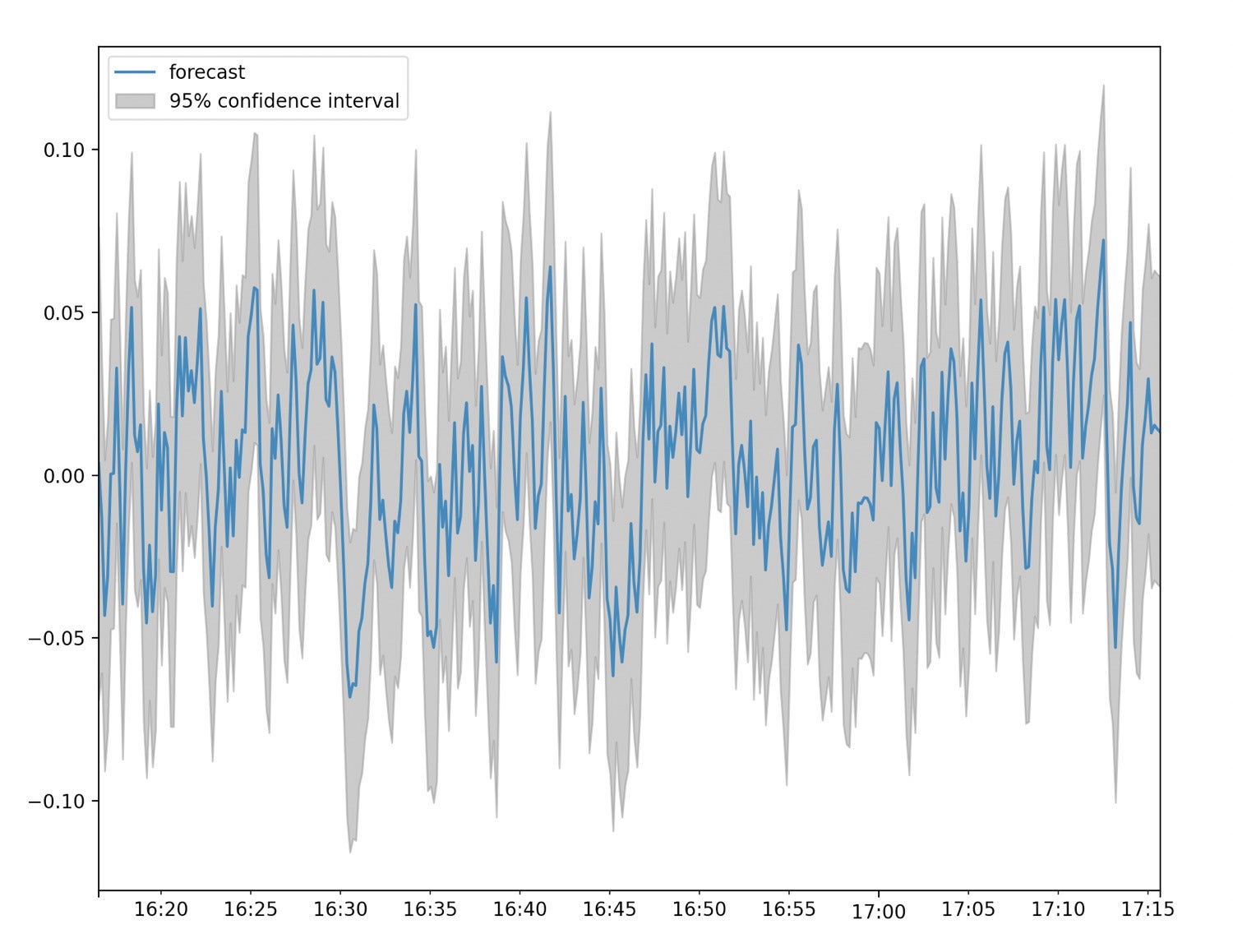InfluxData

The bottom line

I hope this blog post inspires you to take advantage of ARMA and InfluxDB to make forecasts. I encourage you to take a look at the following repo, which includes examples for how to work with both the algorithms described here and InfluxDB to make forecasts and perform anomaly detection.

Anais Dotis-Georgiou is a developer advocate for InfluxData with a passion for making data beautiful with the use of data analytics, AI, and machine learning. She applies a mix of research, exploration, and engineering to translate the data she collects into something useful, valuable, and beautiful. When she is not behind a screen, you can find her outside drawing, stretching, boarding, or chasing after a soccer ball.

—

New Tech Forum provides a venue to explore and discuss emerging enterprise technology in unprecedented depth and breadth. The selection is subjective, based on our pick of the technologies we believe to be important and of greatest interest to InfoWorld readers. InfoWorld does not accept marketing collateral for publication and reserves the right to edit all contributed content. Send all inquiries to [email protected].